This applet provides a 3D representation of the wavefunctions \(\psi_{n,\ell,m}(r,\theta,\varphi)\) of the hydrogen atom.
Using the toolbar, you can specify desired values of \(n\), \(\ell\) and \(m\). The mouse can be used to change the point of view and the zooming factor.
The wavefunction is represented using isodensity surfaces, defined as surfaces where \(|\psi_{n,\ell,m}(r,\theta,\varphi)|\) takes a constant value \(\eta\),
chosen so that there is a probability \(\cal P\) of finding the electron inside the enclosed volumes, where \(|\psi_{n,\ell,m}(r,\theta,\varphi)|\ge\eta\). In other words,
\(
\iiint_{|\psi(\vec r)|\ge\eta} \,|\psi(\vec r)|^2 d^3\vec r = {\cal P}.
\)
The value of \(\cal P\) can be adjusted using the slider in the toolbar.
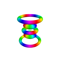
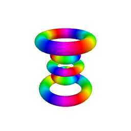
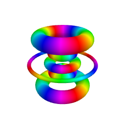
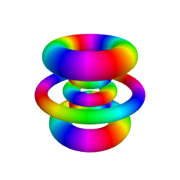
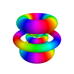
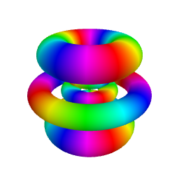
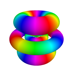
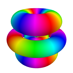
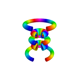
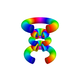
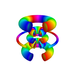
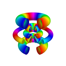
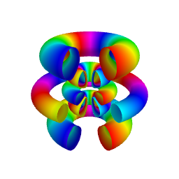
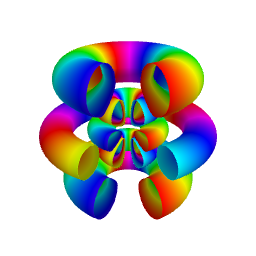
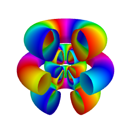
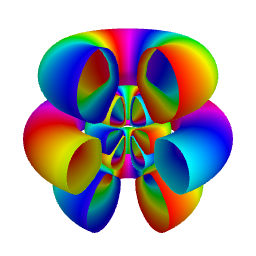
As illustrated in the figure below obtained for \(n=6, \ell=4, m=2\), the isodensity surfaces obtained for different values of \(\cal P\) are the 3D analog of contour lines in
2D representations. Smaller values of \(\cal P\) are associated with greater values of \(|\psi_{n,\ell,m}(r,\theta,\varphi)|\).
| \({\cal P}=0.1\) |
\({\cal P}=0.2\) |
\({\cal P}=0.3\) |
\({\cal P}=0.4\) |
\({\cal P}=0.5\) |
\({\cal P}=0.6\) |
\({\cal P}=0.7\) |
\({\cal P}=0.8\) |
\({\cal P}=0.9\) |
 |
 |
 |
 |
 |
 |
 |
 |
 |
 |
 |
 |
 |
 |
 |
 |
 |
 |
|
The upper row shows the full isodensity surfaces while the lower row corresponds to sectioned views, which can provide a better view of hidden inner surfaces.
The phase of the wavefunction is color encoded using the color code shown on the right.
Finally, you can adjust the number of segments used to compute the surface along meridians and parallels. A greater number of segments provides a higher-quality surface but with a slower update rate.
|

|
Background
Due to the rotation invariance of the problem, the Hamiltonian \(\hat H\) commutes with the angular momentum operator \(\hat{\vec L}\), so that the three
observables \(\hat H\), \(\hat L^2\) and \(\hat L_z\) can be simultaneously diagonalized. When spin is not taken into account, these observables constitute a
complete set of commuting observables, so that the common eigenstates \(|n,\ell,m\rangle\) are unique, with \(\hat H|n,\ell,m\rangle = E_n|n,\ell,m\rangle\),
\(\hat L^2|n,\ell,m\rangle = \ell(\ell+1) \hbar^2|n,\ell,m\rangle\) and \(\hat L_z|n,\ell,m\rangle = m\hbar|n,\ell,m\rangle\). Note that for
the hydrogen atom, the energy \(E_n = -E_I/n^2\) depends only on \(n\), where \(n\in\mathbb{N}^*\). \(\ell\) is an integer such that \(0\le\ell\le n-1\)
and \(m\) is an integer such that \(-\ell\le m\le\ell\).
It can be shown that the wavefunctions associated with these eigenstates read
\(\psi_{n,\ell,m}(r,\theta,\varphi) = R_{n,\ell}(r) Y_{\ell,m}(\theta, \varphi)\)
where \(Y_{\ell,m}(\theta,\varphi) = F_{\ell,m}(\theta)\exp(i m \varphi)\) is a
spherical harmonics.
The fact that \(R_{n,\ell}(r)\) has \((n-\ell-1)\) nodes and that \(F_{\ell,m}(\theta)\) has \(\ell-|m|\) nodes (in the \(]0, \pi[\) interval) allows
to easily recognize any hydrogen orbital, provided you properly adjust the value of \(\cal P\) so as to visualize all relevant volumes and avoid missing
any node of the wavefunction.